What is CBM (Condition-Based Maintenance)?
From IBM’s site: “Condition-based maintenance (CBM) is a preventive maintenance strategy that relies on the monitoring of assets or equipment to determine when maintenance work is necessary.
CBM involves the use of sensors and other monitoring equipment to collect data on the performance of equipment. Using algorithms, machine learning and AI the collected data is then analyzed to identify patterns and anomalies that might indicate a maintenance issue.
In the past, companies only performed maintenance on a fixed schedule or when equipment failed, often resulting in expensive and inefficient maintenance practices (that is, unexpected downtime and emergency repairs). However, condition-based maintenance offers a newer, more advanced approach to maintenance management.
Rather than performing maintenance on a predetermined schedule or waiting for equipment breakdowns, CBM uses real-time data to identify maintenance needs, allowing for more efficient and cost-effective maintenance practices.”
A new approach to CBM is offered by QCM (Quantitative Complexity Management) technology. It too reads the outputs of sensors, however, contrary to mainstream thinking, it:
- does not need Machine Learning
- is able to identify anomalies that are very rare and which cannot be used by Machine Learning algorithms
- is able to measure the State of Health of an entire system, comprising tens of thousands of sensors, in real time
- produces new parameters that are key for modern CBM
These parameters are:
- Accumulated Activity (AA)
- Usage Intensity (UI)
- Degradation Index (DI)
The AA measures how much a component has been used and it may be seen as a sort of ‘mileage’ or ‘travel distance’. The Usage Intensity measures how intensly the ‘mileage’ has been covered. Imagine driving for a 1000 miles in a city, or on a motorway. The distance is the same but the stress on the engine is different. Imagine driving the same 1000 miles at 50 mph or at 80 mph. Both AA and the UI are able to make the distinction.
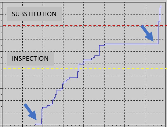
In the present blog the Degradation Index will be illustrated. As the name suggests, it measures the amount of wear and tear of a particular component and it’s evolution over time reflects the history of said component. An example is shown below:
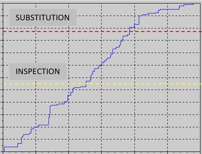
The yellow and red dashed lines show, respectively, two levels of maintenance. Once the yellow line is crossed one knows that the component will soon need to be substituted or serviced. This particular example is that of a component with a fairly constant rate of wear and tear, which starts on day one of operation.
Another example, in which degradation is triggered by an anomaly, is illustrated below:
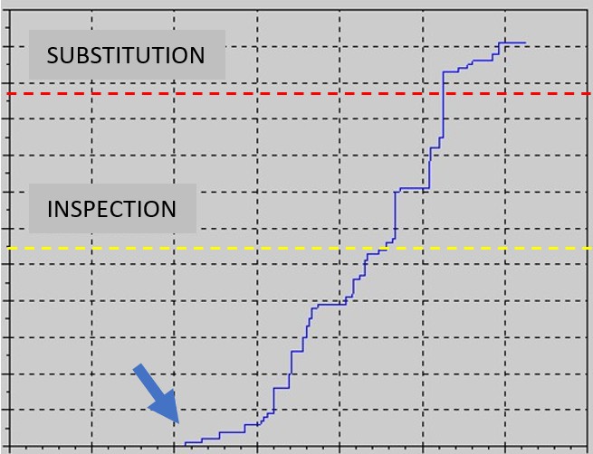
The arrow indicates the presence of an anomaly which initiates degradation, which may proceed at different rates once it commences. The next example is very similar, except that degradation is very fast and characterised by strong gradients.
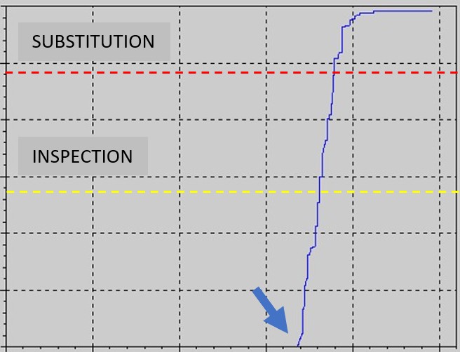
The last example is a combination of the previous cases, except that a second anomaly accelerates the final phase of the degradation process, leading to component substitution or repair:
The Degradation Index is computed based on all the sensor outputs a given component is able to produce and obviously is computed in real-time.
In highly complex scenarios, such as large manufacturing or process plants, where there are hundreds of different components or machines, the number of things that can, and that do go wrong, can be immense. Once cannot use Machine Learning to train for the unexpected or for the unknown – ML can only react to what it has been trained to recognise. Before you jump on the AI train, this may be worth a read.
The DI is computed by the CAHMS Microcomputer.
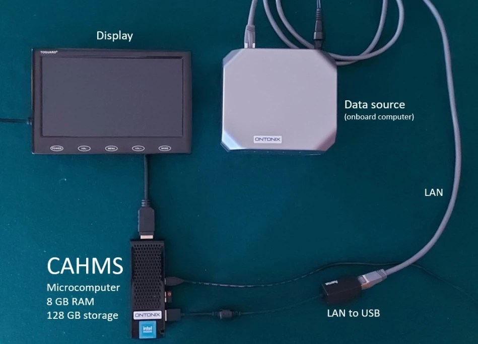
You can read about the CAHMS here.

Pingback: Monitoring Degradation via Complexity – Artificial Intuition