Monitoring Degradation via Complexity

In a recent blog we introduced a new, systemic complexity based Degradation Index. The reason this index is systemic in nature is because it combines all sensor measurements into one single entity – complexity – which reflects the state of health of a system, its accumulated wear and tear and intensity of usage. The other important advantage of this Degradation Index is that it also considers all possible interdependencies between sensor readings. This guarantees that nothing strange goes unnoticed.

However, when monitoring different systems and processes it is important to keep in mind a few key aspects of the physics of the underlying phenomenon in order to avoid mistakes and pitfalls.

All physical phenomena possess characteristic frequences. For example, very low frequencies may be present, modulated by high-frequencies as well as noise. It is crucial to know these frequencies because they mandate the correct sampling frequency of sensor outputs as well as the size of a typical analysis window. Signal Fourier analysis or modal analysis may be performed in order to establish these quantities correctly and avoid loss of information or distorsion. Sometimes, due to degradation, the characteristic frequencies of a system may change, more or less gradually. Imagine a loss of stiffness and load carrying capacity because of corrosion or fatigue. If undetected, this can lead to misinterpretation of results of data analysis.

However, what we wish to address in this blog is a problem of a completely different nature. Imagine that we’re interested in monitoring very slow degradation resulting, for example, from fatigue. Fatigue is a phenomenon that may be very slow (unless accelerated by initial defects or bad design) and take place over periods of years. Imagine a bridge, a train or an aircraft. A bridge, for example, may suffer accelerated degradation because of a single earthquake in its entire operating life. An aircraft can suffer a few hard landings, or badly performed maintenance, which can ultimately lead to fatal consequences.

In the case of freight trains the loading condition on a particular car may vary significantly, due to train length, itinerary, load, etc. This means that degradation of certain components may proceed with varying intensity and speed. This is of course obvious.

The key issue, however, when monitoring very long-term phenomena, is related to the period of monitoring. There are two types of monitoring:

Continuous (realtime) monitoring.
Intermittent monitoring.

In the case of continuos monitoring, data originating from sensor readings is collected at all times. It may be analysed is real time or processed a-posteriori at regular intervals when downloaded into a server. This approach is used when anomaly detection is of interest.

Intermittent monitoring is performed for short periods of time, hours, or days, and data is analysed off-line. The goal may be, for example, to compare the degradation of the same component type on two different cars, see example below.

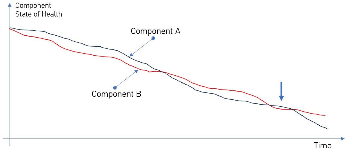
The obvious issue is indicated in the above plot – if performed over short periods of time, a component may momentarily appear as more or less damaged than the other one – see blue vertical arrow.

Consequently, monitoring very slow phenomena over very short periods of time may deliver insignficant and misleading results. This is true for any analysis method. The only reasonable alternative is long-term monitoring.

Moreover, monitoring a very small number of components is also risky because one has no idea of the intrinsic manufacturing and/or assembly variability that is present in every engineering process. At least a few tens of components should be analyzed.