
Proteins are modular in their construction. They are formed by chaining together amino acid molecules, with the smallest amino acid (glycine, C2H3NO) having 7 atoms and the largest (pyrrolysine, C12H19N3O2) having 36.
Depending on how many amino acids there are in a protein (ranging from a few dozen to several thousand), the number of atoms varies immensely.
The smallest known protein is TRP-cage, with only 20 amino acids and 154 atoms.
The most common protein in humans is collagen, which makes up the bulk of our connective tissues. There are several variants of collagen, but the first hit in the RSCB protein data bank has 1408 atoms, so that is a good example of the atom count in a “typical” protein.
Understanding and simulating the protein folding process has been an important challenge for computational biology since the late 1960s.
Ontonix has performed tests with a protein comprised of 435 atoms. Molecular Dynamics simulation has been utilized to determine the position of each of the atoms until the protein has reached its final state. The data has been provided by the CINECA Supercomputer Center in Bologna, Italy.
Molecular Dynamics (https://www.ncbi.nlm.nih.gov/pmc/articles/PMC4655909/) simulation, first developed in the late 70s, has advanced from simulating several hundreds of atoms to systems with biological relevance, including entire proteins in solution with explicit solvent representations, membrane embedded proteins, or large macromolecular complexes like nucleosomes or ribosomes. Simulation of systems having ~50,000–100,000 atoms are now routine, and simulations of approximately 500,000 atoms are common when the appropriate computer facilities are available. This remarkable improvement is in large part a consequence of the use of high performance computing (HPC), and the simplicity of the basic MD algorithm (see figure below).
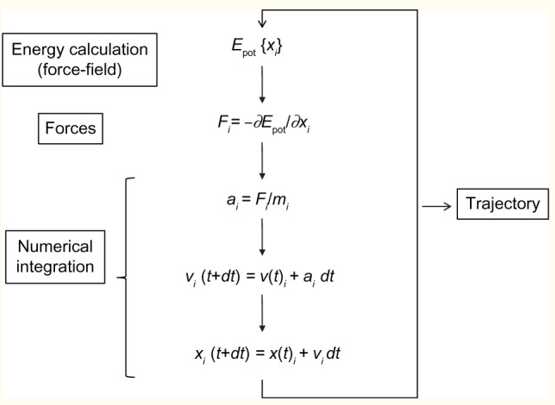
An initial model of the system is obtained from either experimental structures or comparative modelling data. The simulated system could be represented at different levels of detail. Atomistic representation is the one that leads to the best reproduction of the actual systems. However, coarse-grained representations are becoming very popular when large systems or long simulations are required. Several approaches have been assayed but, again, the most effective is the simplest one, the explicit representation of solvent molecules, although at the expense of increasing the size of the simulated systems. Explicit solvent is able to recover most of the solvation effects of real solvent including those from entropic origin like the hydrophobic effect. Once the system is built, forces acting on every atom are obtained by deriving equations, the force-fields, where potential energy is deduced from the molecular structure. Force-fields are complex equations, but they are easy to calculate. The simplicity of the force-field representation of molecular features: springs for bond length and angles, periodic functions for bond rotations and Lennard–Jones potentials, and the Coulomb’s law for van der Waals and electrostatic interactions, respectively, assures that energy and force calculations are extremely fast even for large systems. Force-fields currently used in atomistic molecular simulations differ in the way they are parameterized. Parameters are not necessarily interchangeable, and not all force-fields allow to represent all molecule types, but simulations conducted using modern force-fields are normally equivalent. Once the forces acting on individual atoms are obtained, classical Newton’s law of motion is used to calculate accelerations and velocities and to update the atom positions. As integration of movement is done numerically, to avoid instability, a time step shorter than the fastest movements in the molecule should be used. This ranks normally between 1 and 2 fs for atomistic simulations, and is the major bottleneck of the simulation procedure. Microsecond-long simulations, barely scratching the time scales of biological processes, require iterating over this calculation cycle 109 times. This is one of the strengths of coarse-grained strategies. As a more simplified representation of the system is used, much larger time steps are possible, and therefore the effective length of the simulations is dramatically extended. Of course, this can be obtained at the expense of the accuracy of the simulation ensemble. Algorithmic advances, that include fine-tuning of energy calculations, parallelization, or the use of graphical processing units (GPUs), have largely improved the performance of MD simulations.
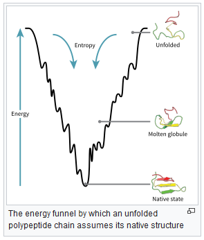
Proteins tend towards their native state, which occupies a (local) minimum energy position in the protein’s energy landscape, see figure below (from https://en.wikipedia.org/wiki/Protein_folding):
Once MD results are available, we can use the QCM tool to track the complexity of the molecule (protein) over time. We have found the following interesting result. The plot represents protein complexity over time.
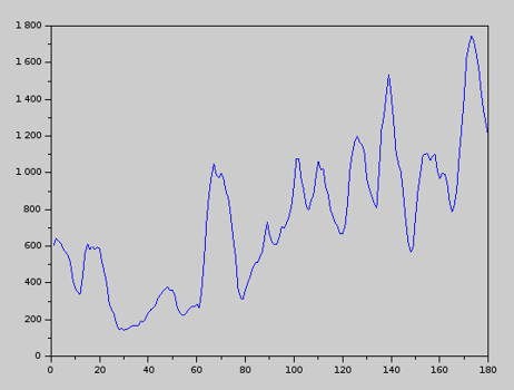
While a protein tends toward a minimum-energy configuration, at the same time it maximizes its own complexity. This makes sense if we recall the definition of complexity: complexity is structured information. The shape of a protein encodes information (the DNA, for example, is a structure that encodes information through the order, or sequence, of the nucleotides along each strand). For a given ensembles of aminoacids, which will ultimately fold into a protein, nature does two things: it minimizes the protein’s energy and, at the same time, it maximizes the amount of information that it can encode with those aminoacids. With all likelihood – this is only a conjecture – the final state of a protein is a compromise (combination) of these two key attributes: energy and information.
The Complexity Map of the 435-atom protein in the vicinity of its final state is shown below. The number of nodes on the diagonal is of course 435 x 3 = 1305, and the number of interdependencies is just under 210 000 while the map density is 25%.

An example of what this map represents is shown below. The first three nodes in the Complexity Map are, respectively, the x, y and z coordinates of the first atom, the following three are those of the second atom, and so on.

While this result needs to be verified by analyzing other proteins, it appears that a minimum energy-maximum complexity (information) state is an ‘obvious’ state which results from the process of folding. Evidently, the more information a protein (or any other system for that matter) contains, the more functions it can perform.
Only as a matter of curiosity, we illustrate below the Complexity Landscape of the 435-atom protein in question. The landscape has dimensions 180 (these are discrete frames used to display complexity and its landscape) by 1305.
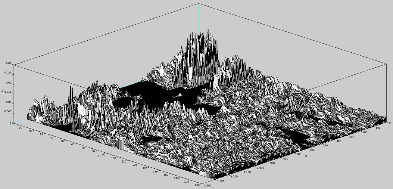
One can notice how in the initial state (frame 1) there were a few ‘dominant’ atoms (top of the figure) while after 180 frames, the complexity contributions are distributed rather uniformly.

0 comments on “The Complexity of Proteins and Protein Folding”