

Robust design (and decision-making) has been a goal for engineers and managers for quite some time now. But what actually is robustness? Can it be measured? There are many definitions of robustness. Let’s see a few of them:
- Robustness is the persistence of specified system features in the face of a specified assembly of insults.
- Robustness is the ability of a system to maintain function even with changes in internal structure or external environment.
- Robustness is the ability of a system with a fixed structure to perform multiple functional tasks as needed in a changing environment.
- Robustness is the degree to which a system or component can function correctly in the presence of invalid or conflicting inputs.
- A model is robust if it is true under assumptions different from those used in construction of the model.
- Robustness is the degree to which a system is insensitive to effects that are not considered in the design.
- Robustness signifies insensitivity against small deviations in the assumptions.
These definitions – the list is by no means complete – are quite popular but they are of little practical use. But when is a definition actually useful?
A definition is of practical use when it hints a metric, a means of measuring something. In fact, serious science started when Galileo begun to measure the outcomes of his famous experiments.
A new and useful definition of robustness, which suggests a metric and which is based on the concept of complexity and graph theory, is as follows:
Robustness is the capacity of a system to maintain the topology of its Process Map (functionality) intact in the presence of endogenous and/or exogenous disturbances.
In order to measure robustness of a system it is therefore necessary to first construct the corresponding Process Map. Consider a dynamical system, described by a set of inputs (see below), outputs, and a mathematical (or physical) model which maps the inputs onto the outputs (Fig. 3.1).
Fig. 3.1: Example of a dynamical system with inputs (left) and outputs (right).
As we know, the input-output relations form a network (a graph) which describes the topology of information flow from within the system (typically this information flows from inputs to outputs – left to right in the picture above). Such flow may be processed by OntoSpace™ to yield the so-called Process Maps. An example, illustrating a mechanical system, is shown below. The red nodes in the Process Map correspond to inputs (left in the above scheme) while the blue ones to outputs (Fig. 3.2 and Appendix 8.2).
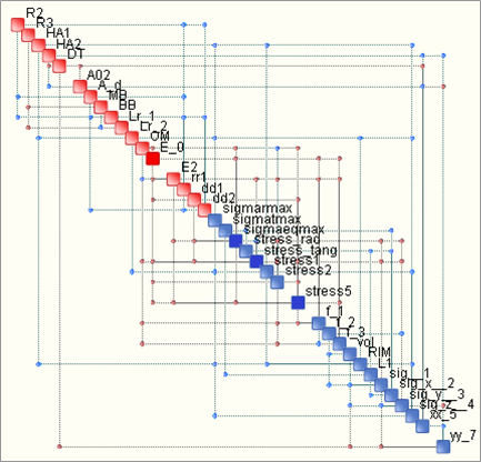
Fig. 3.2: Example of a process map, linking inputs (red) to outputs (blue).
The construction of the Process Map is performed based on the results of a Monte Carlo Simulation in which the inputs are sampled randomly and repeatedly according to prescribed Probability Density Functions (PDFs). The concept is illustrated below (Fig. 3.3).

Fig. 3.3: Formulation of a stochastic problem which may be solved using Monte Carlo Simulation, the results of which are necessary to construct the corresponding process map.
The suggested robustness definition indicates that the functionality of a system is related to the “stability” of its Process Map. It is evident that if the system is properly designed, and produces the desired outputs, it is mandatory to maintain the Process Map intact. In other words, a good design is such that leads to a stable topology of its Process Map. Put in practical terms, when the system is exposed to external (environmental) uncertainties, such as loading or boundary conditions, as well as internal uncertainties, such as assembly imperfections or scatter in material properties, it should still function properly. This means that the functionaly remains intact in the face of the mentioned uncertainties.
Functionality is maintained if the topology of the information flow is maintained. In other words, disturbances and uncertainties will tend to erode the structure of a system’s Process Map. This is in line with the Second Principle of Thermodynamics which illustrates how the inevitable increase of entropy leads to an irreversible process known as aging. Ultimately, agins is equivalent to a progressive loss of functionality. A robust design will resist this decay of the structure of its Process Map so that its topology remains unchanged. For this reason, we refer to this definition of robustness as topological robustness. The “amount of topology” in a Process Map is quantified via its complexity. It is precisely because of the fact that complexity may be used to “measure topology” that we establish a rational link between complexity and robustness. From a practical standpoint, the measure of robustness may be quantified as the Process Map’s sensitivity to increments of entropy. This is because increasing the entropy of a system may cause loss of structure – in effect, if one increases the amount of noise on top of information transmission between two nodes (components of a network) the transmission may eventually become so noisy that no useful information is sent from one node to another. In other words, the link is broken, affecting the map’s topology. In most cases, this leads to loss of functionality or, in the best of cases, to loss of redundancy. Therefore, we propose the following measure of topological robustness:
R = exp(-dC/dH)
where C stands for complexity and H for entropy.
The term in parentheses represents the sensitivity of the complexity of a Process Map to changes in entropy. Use of the exponential function guarantees that when the sensitivity is infinite, R=0, when the sensitivity is 0, R=1.
The quantification of robustness according to the above formula is computationally expensive, so we replace it with an approximate approach which is based on the distance of a system from its critical complexity. The concept is illustrated below (Fig. 3.4).
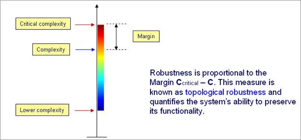
Fig. 3.4: Topological robustness as function of current and critical complexity of a system.
In order to understand better the mechanism behind the computation of topological robustness it is necessary to introduce the concepts of lower and upper complexity bounds in dynamical systems. Imagine that a Monte Carlo Simulation is performed or, eqivalently, certain measurements from a set of sensors are collected from a given system. Suppose also that two situations are analyzed, which differ in terms of how much noise is transitted between the various system components. Clearly, systems that are assembled according to stringent quality requirements are generally “less noisy”, while low-quality products are quite the opposite. Supposing that in both cases the topology of the Process Maps are identical, the more noisy case will correspond to a more complex situation. This is illustrated below (Fig. 3.5).
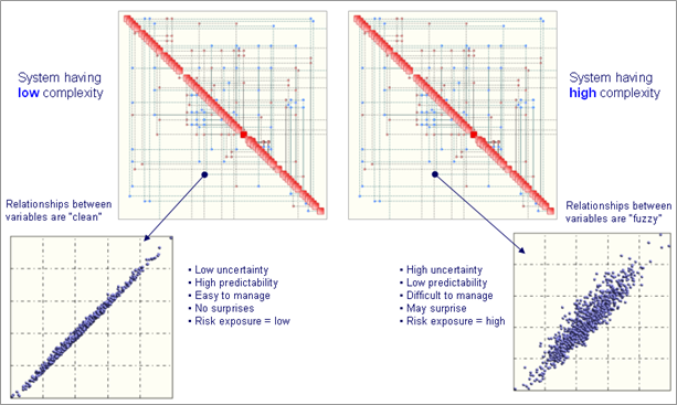
Fig. 3.5: Process Maps of a given system in which two different levels of noise are tansmitted. The situation could correspond, for example, to a high-quality (left) and low-quality (right) assembly/manufacturing process. This is evident in the two scatter plots reflecting a typical relationship between variables.
In the case having higher noise content the system is also more complex. Fuzzier relationships between variables (components) reflect a higher entropy content in the system – see the scatter plot on the right hand side in figure 3.5 – and indicate a more aged system. Complexity – which is a function of the Process Map’s topology and entropy – is consequently higher and the system is generally more difficult to manage in that higher complexity implies the capacity of the system to deliver surprising or unexpected behaviour.
As a system ages, the erosive action of entropy is evident via a progressive “softening” of the relationships between variables (components). In other words, a typical relationship will transition from a “clean” one (not necessarily linear) like the one on the left in figure 3.5, to one which resembles the one on the right in the same figure. As time progresses, most, if not all relationships between variables become less and less crisp and the system becomes less predictable, hence more difficult to manage. In practice this means that the system may perform in an unsatisfactory manner or even suddenly change the way it behaves. This last phenonemnon is known as spontaneous mode-switching and is generally very undesireable.
The upper complexity bound – known also as critical complexity – corresponds to that value of complexity which has been computed assuming that all of the relationships in a Process Map are on the verge of collapse. In other words, all scatter plots are close to being “chaotic” and the system, as a whole, is also on the verge of chaos. Conversely, the lower complexity bound is computed assuming that all relationships are crisp. The system, in such a situation, behaves as a totally deterministic system. Both extremes are illustrated below (Fig. 3.6).
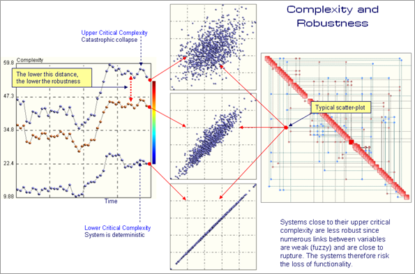
Fig. 3.6: Evolution of a dynamical system. The plot on the left illustrates the time-history of the system’s complexity (orange curve) as well as the lower and upper complexity bounds. A typical scatter plot is shown as well as the topology of the system’s Process Map. Sudden changes in the system’s complexity indicate traumatic events which may have endogenous or exogenous causes.
At this point it becomes clear how the concept of topological robustness is related to complexity. When close to the lower complexity bound, the system behaves in a deterministic fashion and small increments of entropy (noise) will not perturb the various relationships (scatter plots) between variables to cause changes in the Process Map’s topology. In other words, the map’s topology remains intact. This guarantees that functionaly remains intact. If, on the other hand, some relationship in the system are extremely “fuzzy” (or chaotic), even a small increment in entropy may cause this relationship to disappear, making communication between components impossible. Imagine radio transmission which is very noisy but in which one can still make sense of the information that is being transmitted. There is a point at which adding more noise it becomes impossible to receive useful information. The link is broken, functionality is compromised. In mechanical systems the analogy is simple. Think of a bearing, or a spring, that rusts and ultimately brakes, failing to connect two components or creating such mechanical play between components that they no longer perform correctly. This is precisely what happens in proximity of critical complexity. From a functional standpoint, topological robustness may be expressed as follows:
R = f (C; CL; CU)
where C, CL and CU stand for, respectively, the current system complexity, lower and upper bounds. The function is such that:
If C = CL, R = 1
If C = CU, R = 0
The function is such that R drops quickly as C approaches CU.
Process maps, however, can be an important source of additional and significant information about a given system’s robustness and other vital properties such as redundancy. A fundamental characteristic of a Process Map is the so-called connectivity histogram. Such histograms reflect how many connections does a particular variable (node of a Process Map) possess with the remaining variables. This number of connections (relationships) is known as degree.
Nodes having the highest degree are known as hubs. An example of a connectivity histogram is illustrated below (Fig. 3.7).
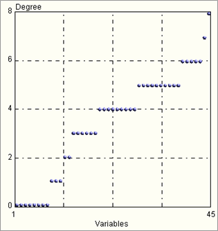
Fig. 3.7: Example of connectivity histogram of a Process Map with 45 nodes. One may notice the existence of one hub having degree of 8 as well as one node with degree 7. Follow 5 nodes with degree 6.
Systems in which the connectivity histogram is very spiky, or sharp, are known as Zipfian (named after the Linguist George Kingsley Zipf). Such systems are known to be fragile, in that a Zipfian distribution points to the existence of a hub, or very few hubs, which have degree far greater than the majority of the nodes in a given network. This means that the loss of that particular node (hub) will have disastrous effects on the entire network. Flatter distributions, on the other hand, point to systems which are less sensitive to the loss of a hub and are generally less fragile and more difficult to destroy. Below we indicate two different designs to a mechanical problem, which have very similar values of topological robustness (approximately 80%) but which have marked differences as far as the connectivity histograms are concerned (Fig. 3.8).
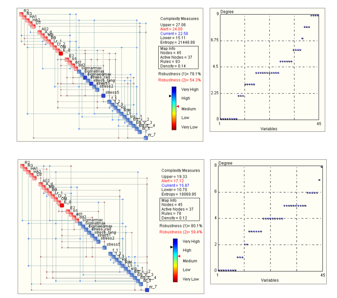
Fig. 3.8: Example of two different solutions to a mechanical design problem. Both solutions have very similar topological robustness – approximately 80% – the lower one, however, has a more spiky connectivity histogram.
In general, designs with Zipfian distribution should be avoided. Such single-hub systems are inherently fragile. An analogy from biology illustrates the concept very clearly. Ecosystems in which only one hub in the food-chain is present are fragile in the case hub comes under attack. Such hubs are known as “keystone species” and are often represented by an innocent incent of vertebrate. However, removal of such a species can quickly bring the entire ecosystem to catastrophic collapse if it cannot adapt quickly enough.
However, one must distinguish also the following two situations:
- Random attack
- Targeted attack
Suppose that one randomly “shoots” at a given system. If the system has only one hub, the probability of hitting it under random fire are small, precisely because we only have one hub. If more hubs are present, the chance of hitting a hub are of course greater. In the case of a targeted attack it is of course better to dispose of more hubs as it will take more time to shoot them all down. Therefore, one has to be careful when stating that a Zipfian system is more exposed. This may or may not be true. In other words, each case has to be examined carefully.
In the case of mechanical systems, such as cars, satellites, or aircraft, the “attack” is essentially random but it is also distributed, i.e. “many bullets” are fired at the system, not just one. Corrosion, creep, erosion, seepage, fatigue, wear, etc. act at the same time in every corner of a complex system. The process of aging, consequence of the Second Law of Thermodynamics, is inexorable and quite “democratic” – it spares no one.
A final contribution towards the understanding of how a system will respond in its interaction with the surrounding environment may be found in the Process Map’s density. Density of a map is defined as:
D = 2 L/[N*(N-1)]
where L stands for the number of links (relationships) and N the number of nodes in a graph (Process Map). Generally speaking, a high value of density corresponds to systems with a high degree of redundancy. In other words, information from node to node may be transmitted in a multitude of ways, using different paths. If one path fails, others are available – this is precisely the concept of redundancy. Systems with a high density have, consequently, a higher degree of controllability as well as observability.
Topological robustness, due to the fact that it addresses the Process Map of a given system, is a global measure of robustness. Let us now look into more detail into the issue of robustness from a one and two-dimensional perspective. In other words, we will investigate the case of only two variables. This will help to appreciate better the concepts described above.
First of all, let’s focus on the simple “scalar” definition of robustness. The commonly accepted definitions of robustnees mistakenly state that a system with low scatter in performance is robust. We state that a single-degree of freedom system behaves in a robust manner if its probability density function (PDF) is uni-modal. When the PDF is multi-modal – see figure below (Fig. 3.9) – the system (in the case of a particular variable or channel) can spontaneously jump from one peak (mode) to another.
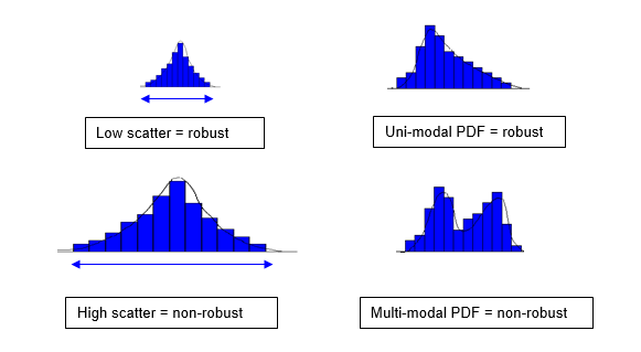
Fig. 3.9: Incorrect (left) and correct (right) definitions of robustness. Low or high performance scatter points to high or low quality, respectively, and has little to do with robustness. Robustness is related to the character of the distribution, not to its spread.
Uni-modal distributions indicate systems which, for a particular channel, have only one most-likely response, or behaviour. In bi-modal or multi-modal distributions, a system can spontaneously deliver two distinct most-likely modes of behaviour. Therefore, one may see the departure from an equivalent Gaussian (uni-modal) distribution as a measure of simple, or scalar, robustness. The presence of multiple peaks in a PDF indicate clustering which, in turn, points to bifurcations. The fact that there exist clusters points to discontinuities or other pathologies in the input-output mapping. An example, shown in the figure below (Fig. 3.10), indicates how a rectangular region of the input space, when sampled uniformly is mapped onto a discontinuous domain in the output space. The white circle indicates an area of the output space where a bifurcation is present. This means that small changes in the values of the inputs may place the response on one of the two branches within the white circle. This may mean that the system changes behaviour or mode of operation. Evidently, such situations must be avoided.
The presence of clusters, or other discontinuities, indicates often that one is operating in a non-convex domain. A domain (set) is convex if a segment joining any two points lying within the border of the domain is contained entirely within that domain. Clearly, the output domain indicated in the figure below does not satisfy this condition, hence it is non-convex. We claim that non-convex domains are the primary source on non-robust behaviour.
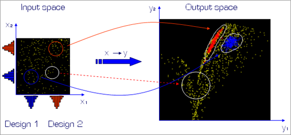
Fig. 3.10: Example of input-output mapping obtained via Monte Carlo Simulation. The white circle indicates a non-convex area of discontinuity in the output space which should be avoided.
It becomes clear, at this point, that the amount of scatter does not point to robustness. It merely indicates quality. In other words, a high-quality product will exhibit small scatter in its operation. This means that any two products taken off the assembly line will be very similar in performance. Low quality, on the other hand, will be reflected in a non-repeatable delivery of performance or characteristics. The concept is summarized in two dimensions in the figure below (Fig. 3.11).
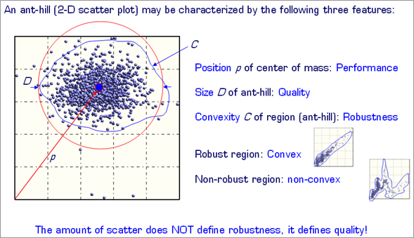
Fig. 3.11: Basic properties of a two-dimensional scatter plot: position, size and convexity.
In figure 3.11 the basic properties of a two-dimensional scatter plot (known also as ant-hill plot) are indicated. These are:
- Position of the centre of mass – this indicates the most likely performance of the system.
- Radius of the circle in which contains the domain – this is proportional to scatter and therefore reflects the quality of the system (if the two dimensions are relative to output parameters).
- Convexity of the domain – this is the property of the 2D domain which reflect the robustness of the system and its ability to spontaneously switch mode of behaviour.
A comparison of two systems operating in a non-convex and convex domain is illustrated below (Fig. 3.12).

Fig. 3.12: Comparison of the properties of a non-convex (left) and convex domain (right).
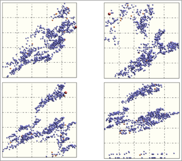
Fig. 3.13: Examples of highly pathological non-convex output spaces. In such cases usage of statistics, interpolation Design Of Experiments or response surface methods doesn’t apply.
Two-dimensional images, such as the ones illustrated in figures 3.10 through 3.13 correspond of course to the relationships linking any two nodes of a Process Map. Since highly non-convex domains will generally point to higher entropy, it is clear that overall system complexity will also increase. It must however be mentioned that convex systems can also lead to multi-modal PDFs. Two examples are shown below (Fig. 3.14).
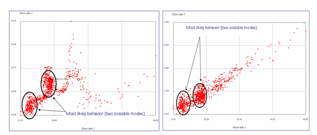
Fig. 3.14: Non convex (left) and convex (right domain). Even though the domain on the right is convex the presence of clusters suggests that multi-modal PDF can still be present if one considers the variables separately. In other words, convexity is not guarantee of uni-modal distributions (PDFs) of the output variables of a given system. The topological robustness concept discussed earlier, measures the distance to catastrophic collapse. This is because by catastrophic collapse we mean total loss of topology in the system’s Process Map. In other words, the map has no connections, and is represented by a set of unconnected nodes. No structure implies no functionality if by functionality we mean transport of information between nodes. Clearly, catastrophic collapse is a very severe situation in which many systems will probably never function.

0 comments on “Background Concepts of Robust Design”