
Consider an enemy network or infrastructure, such as the one shown below. The network is composed of around fifty assets. It could be an energy distribution or a telecomunication network. Suppose the network must be destroyed or crippled in the context of Offensive Cyber Operations (OCO) or in a more conventional strike using ground or airborne assets. The question is where to strike and when to strike.
However, in this blog we address the equally important issue of measuring the effectivness of the strike, i.e. the goal is to measure damage. This will be done from a systemic perspective using QCM technology.
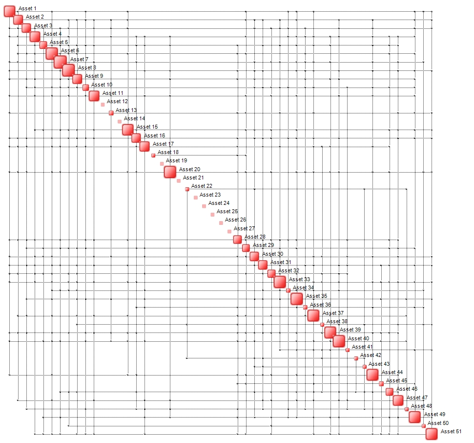
Let us also suppose that the network has been under observation for a certain period of time and it has been determined that its peak complexity is just over 82 Mbits. The density of the network is 64%. This is a high value of density and means that damage propagation (contagion) throughout such a system should be pretty fast. The network also contains numerous hubs (larger boxes on map’s diagonal). This means that there are plenty of good candidates for attack to choose from. In essence, according to QCM (i.e. according to the capacity of a network to carry information) the best moment to strike is at its peak complexity.
Depending on the available energy budget, a strike is delivered. In practice, a certain number of hubs (nodes) is attacked. The result is a crippled network which does, however, retain some residual functionality. The damaged network is illustrated below.

Complexity has dropped to 24 Mbits, while density is now 21%. The number of hubs is now substantially lower than in the pre-strike configuration. Targeting Assets 29 and, say, 42 or 43 should finish things off.
The chart below shows how the complexity of the network increases from an initial value of just under 60 Mbits. After approximately 20 minutes a strike is delivered when peak complexity is attained (82 Mbits). After one hour and forty minutes, the network complexity is down to 24 Mbits. It does try to recover (see t=60 and 90) but after t=115, the system collapses to its final value of 25 Mbits.

The question now is:
What is the amount of damage?
When it comes to destroying complex critical infrastructures or large networks, it is not easy to determine the degree of damage after the strike has been delivered. One simple way to measure damage is to compute the complexity ratio between the pre and post values:
Damage_c = 1 – C_pre/C_post = 1 – 24/82 = 71%
An alternative is to use network density:
Damage_d = 1 – C_pre/C_post = 1 – 21/64 = 67%
A more comprehensive means of damage assessment is to compare not only the map complexity or densities but to compare the entire topologies of both maps. This can be done using OntoTest. Without going into the details of how this is done, the result is as follows:
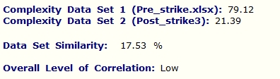
OntoTest measures the degree of similarity of two data sets – in this case pre and post strike data sets are compared. It is found that the degree of similarity (correlation) is low, around 18%. This means that:
Damage_t = 1 – 18% = 82%
This is the true amount of damage that has been inflicted. In order to find out how the damage has actually been distributed, it is sufficient to examine the Delta Profile, shown below:
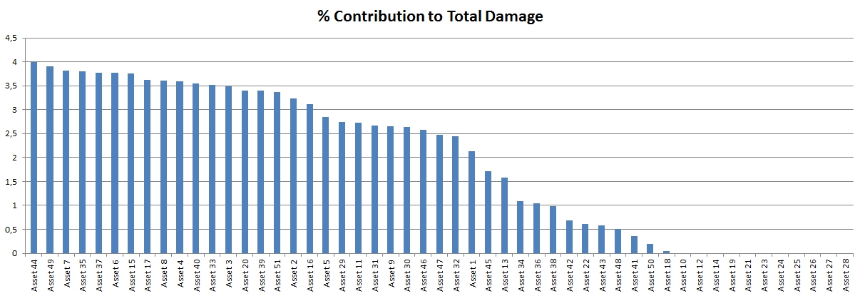
Crippling or destroying Asset 44 induces 4% of the total damage. A additional 3.8% is contributed by Asset49, etc. Other Assets, such as 10, 12, 14 or 19 do not contibute to any systemic damage of the network. This means that targeting them may not have been a good idea.

0 comments on “QCM-based Post-Strike Damage Assessment”