On Stochastic Model Validation

Stochastic validation techniques have been addressed for the first time in the framework of the EU-funded HPCN-Stochastic Correlation of Analysis and Test project, EP24900, in the period 1997-99. The project has been initiated and led by J. Marczyk in 1996. The project has developed innovative metrics and stochastic methodologies for actually quantifying the level of credibility of a numerical model, particularly for cases when multiple solvers are used to attack multi-discipline problems.

Use of a model or simulation is a surrogate for experimentation with an actual system (existing or proposed), where experimentation with that system could be disruptive, not cost effective, or infeasible. If the model or simulation is unable to provide valid representations of the actual system, any conclusions derived from the model or simulation are likely to be erroneous and may result in poor decisions being made.

Validation can be performed for all models and simulations, regardless of whether the corresponding real-world system exists in some form or will be built in the future. Validation should always be focused on the intended use. A precise definition of validation is:

Validation is the process of determining the degree to which a model or simulation is an accurate representation of the real world from the perspective of the intended uses of the model or simulation.

Accuracy in the above definition is intended in statistical sense. Other definitions of model validity are:

1. “Validation means that a model is acceptable for its intended use because it meets specified performance requirements.”
2. “A valid model has no behavior which does not correspond to system behavior.”
3. “We may achieve some of the objectives of a model without validating it.”

The following are different phases of model validation (in the context of simulation):

1. Conceptual validation – checks the soundness of the concept, the logic and the consistency of a model.
2. Operational validation – examines if the model can answer the question it is
   supposed to answer.
3. Quantitative validation – examines to what extent model bahaviour fits the
   observed real system.

The following are some general perspectives on validation:

1. Conceptually, if a simulation is “valid,” then it can be used to make decisions
   about the system similar to those that would be made if it were feasible and
   cost effective to experiment with the system itself.
2. The ease or difficulty of the validation process depends on the complexity of
   the system being modelled and on whether a version of the system currently
   exists
3. A simulation of a complex system can only approximate the actual system, no matter how much time and money are spent on simulation construction.
   There is no such thing as absolute simulation validity, nor is it even desired.
   Indeed, a model or simulation is supposed to be an abstraction and simplification of reality. However, the most valid simulation is not necessarily the most cost effective. For example, increasing the validity of a simulation beyond a certain level might be quite expensive, since extensive data collection may be required, but might not lead to significantly better insight or decisions.
4. A simulation should always be developed for a particular set of objectives.
   Indeed, a simulation that is valid for one set of objectives may not be for
   another set of objectives.
5. The measures and acceptability criteria (e.g., measures of performance) used
   to validate a simulation should include those that the decision-maker will
   actually use for evaluating system configurations.
6. Validation of a stand-alone simulation is a process that should be conducted in coordination with the development or modification effort. It is not something to be attempted after the simulation has already been developed (or modified) and then only if there is time and money remaining.
7. A federation of models still has to be validated even if the models (federates)
   that compose it are believed to be valid.

Conventional model “validation” is based on the attempt to match, as closely as possible, the results of a deterministic numerical analysis, with that of a single physical test. When the distance between the model and the experimental result is sufficiently “close”, the model is said to be valid. However, in statistical terms, this process can only verify (or falsify) a model, and not validate it. In effect, although the process is commonly referred to as “correlation”, it is merely a comparison. Validation in rigorous statistical terms requires a much more complete procedure. First of all, validation of a model, or a theory, must be performed via a repeatable experiment. The experiment is designed in a way that
any other individual may perform it independently and confront the results with the previously made claims. Repeatability is therefore the fundamental requirement of model correlation. Now, due to the fact that uncertainty exists in the material parameters, the loads, the boundary conditions, and assembly tolerances (the list is by no means exhaustive), it is virtually impossible to reproduce any mechanical test within arbitrarily low levels of precision (or resolution). In effect, when uncertainty comes into play, the test is no longer a single experiment, but rather a collection of tests, whose statistical characteristics, such as mean and standard deviation, are indeed repeatable.

Therefore, in an uncertain setting, the test is a collection of tests. This collection is known as meta-model. Clearly, meta-models can also originate from computer simulations. Their complexity can be considerable, and their understanding is paramount towards the comprehension of the behaviour of the system in question. A generic and approximation-free manner of generating meta-models, apart from repeating physical experiments, is via Monte Carlo Simulation. Various commercial codes are available for the purpose, such as MSC.Robust Design, iSight, BossQuattro, LMSOptimus and ST-ORM.

One may identify the following reasons for lack of matching between model and test:

1. Incorrect modelling techniques (e.g. choice of element type)
2. Scatter is neglected
3. Model lacks physics
4. Errors and/or noise in testing

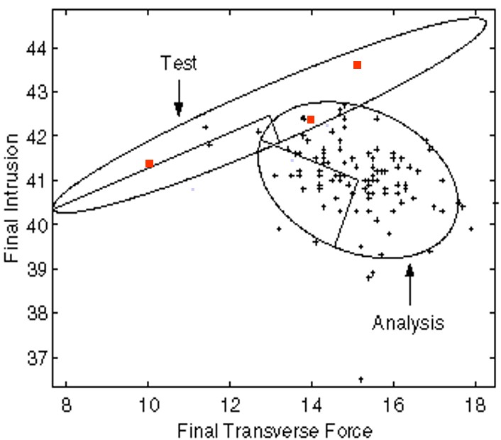
Conventional model-test comparison is normally performed without taking into account parameter scatter. This approach often leads to optimistic results, and may induce one to think that good matching exists. In fact, the smaller the number of parameters that are used for model tuning, the higher the probability of falling into fortuitous conditions reflecting non-existent matching. Experience shows that in order to reduce the chances of “lucky” or false comparison, it is necessary to randomise as much of the model as possible (i.e. to include all the known sources of uncertainty) and to use a large number of parameters for the model tuning process. Therefore, while attempting model improvement or validation, it is necessary to include scatter/uncertainty in the following:

1. Material properties (especially for composite materials)
2. Joint properties (bonding, rivets, bolts)
3. Loads
4. Boundary conditions
5. Assembly tolerances
6. Shape/geometry imperfections (random fields)

However, even before introducing the above sources of uncertainty in the model, it is necessary to first make the model immune to the modelling process itself. In many cases, it has been observed that computed response clouds change shape when one changes, for example, mesh size, time-step-size, algorithm type, computer, solver, etc. Monte Carlo Simulation can help to identify the regions of these “non-physical” quantities where their changes will not be reflected in the meta-model’s statistical properties. Once these regions have been identified, one can proceed to concentrate on physics.

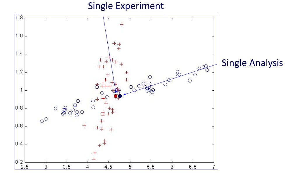
Figure 1 shows an example of a commercial finite element code in which solver-specific parameters have been varied using a Monte Carlo approach, and how these variations influence the results in terms of physical quantities of interest. Before proceeding to validate a numerical model it is therefore necessary to select those values of the non-physical parameters that do not influence the results. The problem of propagating non-physical (i.e. solverspecific) uncertainties in ensembles of computer codes, used for multi-discipline problems, is extremely important. However, it is rarely approached in the industry due to the fact that the necessary methodologies are not well known.

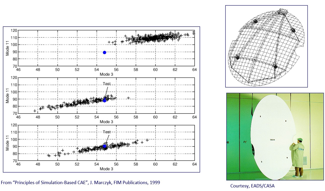
A common problem that often appears in model validation is that only one physical test is available. In this case, given that the covariance information for the experimental metamodel is missing (the meta-model collapses to a single point in N dimensions, where N is the number of measured quantities), all that can be achieved is to position the synthetic meta-model so that its point of highest density (i.e. the most likely response) is located directly on top of the measured response. Clearly, there is no need to orient the metamodel in any particular way, since no information in respect is available.

Other issues that impact model validity/validation to a large extent are:

1. Impact of sensor and actuator placement (often incorrect sensor and/or actuator placement may inhibit the excitation or measurement of certain modes/responses)
2. Definition of significant output quantities (e.g. spectral radius of effective modal mass matrices)
3. Impact of non-linearity.
4. Impact of modelling techniques (experience from the automotive industry shows that wrong finite element choice may induce large mismatch of meta-models)
5. How to make the most of a single test (ideally, model validation is performed
   with two meta-models)
6. Computation of the confidence levels of model-test matching (i.e. probability that the obtained correlation, in case it exists, it real, and not due, for example, to insufficient sample size)

Experience indicates that stochastic model validation provides precious information as to the selection of appropriate modelling techniques (element type, time-step size, joint modelling, etc.) and not merely the forcing of a meta-model to occupy a certain position in the output space. In fact, stochastic model validations yields as by-product, a set of generally valid modelling rules.

Figure 1. Example of how changes in solver-specific parameters may affect simulation results. The quantity on the horizontal axes corresponds to a penetration penalty used to define contact in a commercial crash analysis code. The vertical axes represent physical response quantities. It is clear that in some cases it is possible to select values of penalty that do not influence the results, while in other cases it is not. The scatter of the physical quantities is in certain cases conspicuous.

www.ontonix.com