

Why do most theorems in maths start by saying “let f(x) be a continuous differentiable function…”? Why do so many theorems in statistics assume a normal distribution? Why is it that in mechanics we tend to speak of small-amplitude oscillations around a position of equilibrium? Why is it that we neglect anything that has “epsilon squared” in front of it (just because “epsilon” is usually small – by the way, think of what thousands of small epsilons can do to you if they all work in the same direction!)? The answer is simple. It makes things a lot easier. Theorems with a linear look and feel are easier to prove. When a linear approach is taken, closed-form solutions to numerous problems may be found. Such solutions are said to be elegant and for the sake of elegance one often bends reality to suit his tools. A form of modern art.
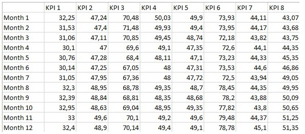
Outside of the scientific realm, similar things take place. Managers identify the so-called KPIs (Key Performance Indicators) and build cost functions whereby the said KPIs are combined using weights or scoring systems. Typically things look more or less like this. A number of KPIs are sampled at, say, monthly or quarterly intervals, as indicated in the array below.
A cost/performance function is then built. Typically, it looks like this:
J = w1 x KPI 1 + w2 x KPI 2 + w3 x KPI 3 + …..+ wN x KPI N (1)
which is a plain vanilla linear combination of the various KPIs. Weights are chosen based on ‘experience’, intuition, ‘expert opinion’, or during long discussions at meetings. These weights often remain unchanged for long periods of time. There seems to be nothing wrong with this classical ‘silo’ approach approach.
However, one very big assumption is hidden in the above cost function, namely that of independence of the KPIs. The formula asserts that all KPIs are independent of each other. And nobody cares to check if this is indeed so.
In reality, most problems we face are, generally, related to other problems. Because things today are becoming highly interdependent – think of the economy for example – it is quite unlikely that also the KPIs reflecting a large corporations would be totally uncoupled. Therefore, the cost function could look like this:
J = w1 x KPI 1 + w2 x KPI 2 + w3 x KPI 3 + …..+ wN x KPI N + a12 x KPI 1 x KPI 2 + a13 x KPI 1 x KPI 3 + …. (2)
where the terms in italics reflect the said inter-dependencies. The above equation is still an approximation because one could introduce higher-order terms such as b1 x KPI 1^2, for example. But for the sake or argument, let’s just stick with equation 2. This equation reflects the structure of inter-dependencies of the KPIs which is clearly apparent in the Complexity Map depicted below. The map has been constructed based on a set of 20 KPIs.

The size of the nodes in the map is proportional to how much complexity each KPI contributes to the system – this, by the way, suggests a new way of assigning weights. However, complexity is not the issue here. The issue is that even in such a simple case there are over 80 inter-dependencies between the 20 KPIs and that these are neglected. Why? Because it is not easy to determine them. So they are simply not accounted for. This minimum-effort approach leaves us with equation 1. Once again, linear thinking attempts to force a warped perception of reality onto a flat, simplistic model. Ignoring the couplings between the KPIs is like saying that the structure in the above map is reduced to this: a list of independent indicators

It is important to know the structure of the inter-dependencies between KPIs. The inter-dependencies that the economy creates will inevitably spillover into the business of any large corporation. Therefore, knowledge of the structure of these inter-dependencies is crucial. Moreover, it is also important to know how much this structure is stable and resilient. Why? Because if the KPIs have been chosen properly – that is if they really are the key indicators – then they really reflect a business. If the structure of the above Complexity Map is stable and resilient, there is a good chance that the same may be said of the business they represent.
The current crisis is obviously very broad, very complex and deep. It may be a very long time before the economy is back on track (whatever that means today). However, it definitely won’t happen if we don’t realize that the world is non-linear, that it is not flat, and that it is turbulent and interconnected. Second, we must realize that old tools and old ways of thinking, that contributed to this global mess, are no longer applicable. If we insist on using outdated philosophies and tools, if we think in linear and ‘three-dimensional’ terms, the current state of crisis will persist or even get worse.
PS. In the image at the top of this blog, laminar flow (left) turns into turbulent flow (right). In Computation Fluid Dynamics (CFD) adopting laminar flow models to turbulent flow leads to dramatically wrong results even if the corresponding computer animations may look deceivingly realistic.
Below, examples of how intricate structure can emerge in diverse applications.

Complexity Map animation by L. Genetti.

0 comments on “Why This Crisis Won’t Go Away (Soon)”